开源日报每天推荐一个 GitHub 优质开源项目和一篇精选英文科技或编程文章原文，坚持阅读《开源日报》，保持每日学习的好习惯。
今日推荐开源项目：《老古董 pong》
今日推荐英文原文：《Complexity Theory for Algorithms》

今日推荐开源项目：《老古董 pong》传送门：GitHub链接
推荐理由：这款制作于1972年的游戏《pong》大概最古老的电子游戏之一。

今日推荐英文原文：《Complexity Theory for Algorithms》作者：Cody Nicholson
原文链接：https://medium.com/better-programming/complexity-theory-for-algorithms-fabd5691260d
推荐理由：关于算法的复杂度理论以及如何优化时间复杂度，毕竟谁都不想用冒泡。

Complexity Theory for Algorithms

How we measure the speed of our algorithms

Complexity theory is the study of the amount of time taken by an algorithm to run as a function of the input size. It’s very useful for software developers to understand so they can write code efficiently. There are two types of complexities:

Space complexity: How much memory an algorithm needs to run.
Time complexity: How much time an algorithm needs to run.

We usually worry more about time complexity than space complexity because we can reuse the memory an algorithm needs to run, but we can’t reuse the time it takes to run. It’s easier to buy memory than it is to buy time. If you need more memory — you can rent server space from providers like Amazon, Google, or Microsoft. You could also buy more computers to add more memory without renting server space. The remainder of this article will cover how we can optimize time complexity.

How Do We Measure Time Complexity?

A new computer will usually be faster than an old computer, and desktops will usually be faster than smartphones — so how do we really know the absolute time an algorithm takes?

To measure the absolute time, we consider the number of operations the algorithm performs. The building blocks of any algorithm are if-statements and loops. They answer the questions: (1) When should we do operations? (2) How many times should we do them? We want to write code using as few if-statements and loops as possible for maximum efficiency on any machine.

For analyzing algorithms, we consider the input size n — the number of input items. We want to make a good guess on how the algorithm’s running time relates to the input size n. This is the order of growth: how the algorithm will scale and behave given the input size n.

1. Input 10 items -> 10 ms
2. Input 100 items -> 100 ms (Good, linear growth)
3. Input 1,000 items -> 10,000 ms (Bad, exponential growth)

In the above example, when we input 10 items, it takes 10 ms to run. When we input 100 items, it takes 100 ms — which is good since the growth of our input increased proportionally to the runtime.

However, on the next step, we input 1,000 items, and it takes 10,000 ms. We’re now taking 10 times longer to run relative to the increase in our input size n. Now we have exponential growth of our runtime instead of linear growth. To better understand the different orders of growth, we’ll cover the Big-O notation.

Big-O Complexity Chart

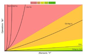The big-o notation describes the limiting behavior of an algorithm when the runtime tends toward a particular value or infinity. We use it to classify algorithms by how they respond to changes in input size. We denote our input size as n and the number of operations performed on our inputs as N. My examples will be coded in Python.

We prefer algorithms that have an order of growth that’s linearithmic in terms of input or faster because slower algorithms can’t scale to large input sizes. Here’s a list of the runtime complexities from lowest to highest:

O(1) : Constant Time Complexity
O(log(n)) : Logarithmic Complexity
O(n) : Linear Complexity
O(n * log(n)) : Linearithmic Complexity
O(n^k) : Polynomial Complexity (Where k > 1)
O(c^n) : Exponential Complexity (Where c is a constant)
O(n!) : Factorial Complexity

Constant Time Complexity: O(1)

An algorithm runs in constant time if the runtime is bounded by a value that doesn’t depend on the size of the input.

The first example of a constant-time algorithm is a function to swap two numbers. If we changed the function definition to take a million numbers as input and we left the function body the same, it’d still only perform the same three operations plus a return statement. The runtime doesn’t change based on the input size.

def swapNums(num1, num2):
   temp = num1
   num1 = num2
   num2 = temp
   return (num1, num2)

In this second example, we’ll first check if the input message is “Hello World!” and change the message to another value if it is. After, it’ll loop three times, executing another loop that’ll print the message 100 times — meaning the message will be printed 300 times total. Despite all those operations — since the function won’t perform more operations based on the input size — this algorithm still runs in constant time.

def printMessage300Times(message):
   if(message == "Hello World!")
      message = "Pick something more original!"
   for x in range(0, 3):
      for x in range(0, 100):
         print(message)

Logarithmic Time Complexity: O(log(n))

A logarithmic algorithm is very scalable because the ratio of the number of operations N to the size of the input n decreases when the input size n increases. This is because logarithmic algorithms don’t access all elements of their input — as we’ll see in the binary-search algorithm.

In binary search, we try to find our input number, num, in a sorted list, num_list. Our input size n is the length of num_list.

Since our list is sorted, we can compare the num we’re searching for to the number in the middle of our list. If num is greater than the midpoint number, we know that our num could only be in the greater side of the list — so we can discard the lower end of the list entirely and save time by not needing to process over it.

We can then repeat this process recursively (which behaves much like a loop) on the greater half of the list, discarding half of our remaining num_list every time we iterate. This is how we can achieve logarithmic time complexity.

def binarySearch(num_list, left_i, right_i, num):
   if right_i >= left_i:
      midpoint = left_i + (right_i - left_i)/2
      if num_list[midpoint] == num:
         return midpoint
      elif num_list[midpoint] > num:
         return binarySearch(num_list, left_i, midpoint-1, num)
      else:
         return binarySearch(num_list, midpoint+1, right_i, num)
   else:
      return "Number not in collection"

Linear Time Complexity: O(n)

An algorithm runs in linear time when the running time increases at most proportionally with the size of the input n. If we multiply the input by 10, the runtime should also multiply by 10 or less. This is because in a linear-time algorithm, we typically run operations on every element of the input.

Finding the maximum value in an unsorted collection of numbers is an algorithm we could create to run in linear time since we have to check every element in our input once in order to solve the problem:

def findMaxNum(list_of_nums):
   max = list_of_nums[0]
   for i in range(1, len(list_of_nums.length)):
      if(list_of_nums[i] > max):
         max = list_of_nums[i]
   return max

In the for loop, we iterate over every element in our input n, updating our maximum value if needed before returning the max value at the end. More examples of linear-time algorithms include checking for duplicates in an unordered list or finding the sum of a list.

Linearithmic Time Complexity: O(n * log(n))

Linearithmic-time algorithms are slightly slower than those of linear time and are still scaleable.

It’s a moderate complexity that floats around linear time until input reaches a large enough size. The most popular examples of algorithms that run in linearithmic time are sorting algorithms like mergeSort, quickSort, and heapSort. We’ll look at mergeSort:

def mergeSort(num_list): 
    if len(num_list) > 1: 
        midpoint = len(arr)//2
        L = num_list[:midpoint] # Dividing "n"  
        R = num_list[midpoint:] # into 2 halves 

        mergeSort(L) # Sort first half 
        mergeSort(R) # Sort second half 

        i = j = k = 0

        # Copy data to temp arrays L[] and R[] 
        while i < len(L) and j < len(R): 
            if L[i] < R[j]: 
                num_list[k] = L[i] 
                i+=1
            else: 
                num_list[k] = R[j] 
                j+=1
            k+=1

        # Checking if any element was left in L
        while i < len(L): 
            num_list[k] = L[i] 
            i+=1
            k+=1
        # Checking if any element was left in R
        while j < len(R): 
            num_list[k] = R[j] 
            j+=1
            k+=1

‘mergeSort’ works by:

Dividing the num_list recursively until the elements are two or less
Sorting each of those pairs of items iteratively
Merging our resulting arrays iteratively

With this approach, we can achieve linearithmic time because the entire input n must be iterated over, and this must occur O(log(n)) times (the input can only be halved O(log(n)) times). Having n items iterated over log(n) times results in the runtime O(n * log(n)), also known as linearithmic time.

Polynomial Time Complexity: O(n^c) where c > 1

An algorithm runs in polynomial time if the runtime increases by the same exponent c for all input sizes n.

This time complexity and the ones that follow don’t scale! This means that as your input size grows, your runtime will eventually become too long to make the algorithm viable. Sometimes we have problems that can’t be solved in a faster way, and we need to get creative with how we limit the size of our input so we don’t experience the long processing time polynomial algorithms will create. An example polynomial algorithm is bubbleSort:

def bubbleSort(num_list):
    n = len(num_list)
    for i in range(n):
        # Last i elements are already in place
        for j in range(0, n-i-1):
            # Swap if the element found is greater
            # than the next element
            if num_list[j] > num_list[j+1] :
                temp = num_list[j]
                num_list[j] = num_list[j+1]
                num_list[j+1] = temp

bubbleSort will iterate over all elements in our list over and over, swapping adjacent numbers when it finds they’re out of order. It only stops when it finds all the numbers are in the correct order.

In the below picture, we only have seven items, and it’s able to iterate over the whole set three times to sort the numbers — but if it was 100 numbers, it’s easy to see how the runtime could become very long. This doesn’t scale.

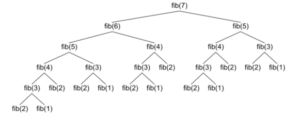
Exponential Time Complexity: O(c^n) Where c Is a Constant

An algorithm runs in exponential time when the runtime doubles with each addition to the input dataset. Calculating the Fibonacci numbers recursively is an example of an exponential-time algorithm:

def fibonacci(n): 
    if n == 0:
        return 0
    elif n == 1:
        return 1
    else: 
        return fibonacci(n-1) + fibonacci(n-2)

This algorithm calls itself twice on the last line — once with n-1 and once with n-2. This means if we started with n=7, we’d call the function a total of 25 times! It’s very expensive to run as the input grows.

Factorial Time Complexity: O(n!)

Lastly, an algorithm runs in factorial time if it iterates over the input n a number of times equal to n multiplied by all positive integer numbers less than n. It’s the slowest time complexity we’ll discuss in this article, and it’s primarily used to calculate permutations of a collection:

def getListPermutation(items_list):
   results = []
   i = 0
   l = len(items_list)
   while i < l:
      j, k = i, i + 1
      while k <= l:
         results.append(" ".join(items_list[j:k]))    
         k = k + 1
      i = i + 1
   print results

Conclusion

Thanks for reading! I’d love to hear your feedback or take any questions you have.

下载开源日报APP：https://openingsource.org/2579/
加入我们：https://openingsource.org/about/join/
关注我们：https://openingsource.org/about/love/

Algorithm

开源日报第751期：《老古董 pong》