每天推荐一个 GitHub 优质开源项目和一篇精选英文科技或编程文章原文,欢迎关注开源日报。交流QQ群:202790710;微博:https://weibo.com/openingsource;电报群 https://t.me/OpeningSourceOrg

今日推荐开源项目:《简单高亮库 Driver.js》GitHub链接
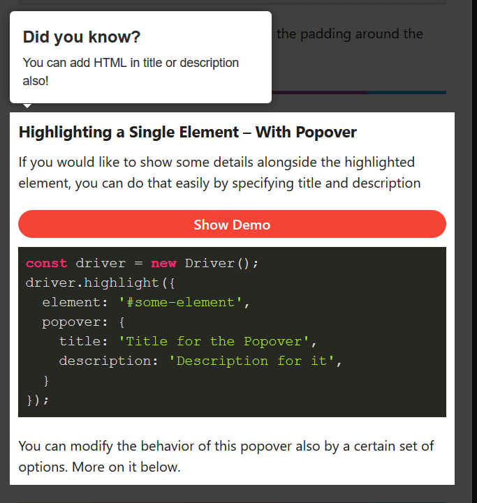
推荐理由:这个库可以让你去高亮某个元素,顺便用各种方法弹出个对话气泡也一样没问题。虽然大部分时候你可能不太需要这个,但是如果你想做个教程之类的或者弄个别的什么比如关灯特效的话,有了这个库肯定能够做的更好更方便。
今日推荐英文原文:《Algorithms in C++》作者:Vadim Smolyakov
原文链接:https://towardsdatascience.com/algorithms-in-c-62b607a6131d
推荐理由:这篇文章顾名思义肯定是讲了 C++ 中的算法的,诸如完全搜索和贪婪算法这些都有介绍,还介绍了不太常见的动态编程,适合正在学习 C++ 的朋友们一看
Algorithms in C++
Introduction
The purpose of this article is to introduce the reader to four main algorithmic paradigms: complete search, greedy algorithms, divide and conquer, and dynamic programming. Many algorithmic problems can be mapped into one of these four categories and the mastery of each one will make you a better programmer.
This article is written from the perspective of competitive programming. In the reference section, you’ll find resources to get you started or improve your programming skills through coding competitions.

Complete Search
Complete search (aka brute force or recursive backtracking) is a method for solving a problem by traversing the entire search space in search of a solution. During the search we can prune parts of the search space that we are sure do not lead to the required solution. In programming contests, complete search will likely lead to Time Limit Exceeded (TLE), however, it’s a good strategy for small input problems.
Complete Search Example: 8 Queens Problem
Our goal is to place 8 queens on a chess board such that no two queens attack each other. In the most naive solution, we would need to enumerate 64 choose 8 ~ 4B possibilities. A better naive solution is to realize that we can put each queen in a separate column, which leads to 8⁸~17M possibilities. We can do better by placing each queen in a separate column and a separate row that results in 8!~40K valid row permutations. In the implementation below, we assume that each queen occupies a different column, and we compute a valid row number for each of the 8 queens.
#include <cstdlib>
#include <cstdio>
#include <cstring>
using namespace std;
//row[8]: row # for each queen
//TC: traceback counter
//(a, b): 1st queen placement at (r=a, c=b)
int row[8], TC, a, b, line_counter;
bool place(int r, int c)
{
    // check previously placed queens
    for (int prev = 0; prev < c; prev++)
    {
        // check if same row or same diagonal
        if (row[prev] == r || (abs(row[prev] — r) == abs(prev — c)))
            return false;
    }
    return true;
}
void backtrack(int c)
{
    // candidate solution; (a, b) has 1 initial queen
    if (c == 8 && row[b] == a)
    {
        printf(“%2d %d”, ++line_counter, row[0] + 1);
        for (int j=1; j < 8; j++) {printf(“ %d”, row[j] + 1);}
        printf(“\n”);
    }
    //try all possible rows
    for (int r = 0; r < 8; r++)
    {
        if (place(r, c))
        {
            row[c] = r; // place a queen at this col and row
            backtrack(c + 1); //increment col and recurse
        }
    }
}
int main()
{
     scanf(“%d”, &TC);
     while (TC--)
     {
        scanf(“%d %d”, &a, &b); a--; b--; //0-based indexing
        memset(row, 0, sizeof(row)); line_counter = 0;
        printf(“SOLN COLUMN\n”);
        printf(“ # 1 2 3 4 5 6 7 8\n\n”);
        backtrack(0); //generate all possible 8! candidate solutions
        if (TC) printf(“\n”);
     }
     return 0;
}
For TC=8 and an initial queen position at (a,b) = (1,1) the above code results in the following output:
SOLN       COLUMN
 #    1 2 3 4 5 6 7 8
 1    1 5 8 6 3 7 2 4
 2    1 6 8 3 7 4 2 5
 3    1 7 4 6 8 2 5 3
 4    1 7 5 8 2 4 6 3
which indicates that there are four possible placements given the initial queen position at (r=1,c=1). Notice that the use of recursion allows to more easily prune the search space in comparison to an iterative solution.
Greedy Algorithms
A greedy algorithm takes a locally optimum choice at each step with the hope of eventually reaching a globally optimal solution. Greedy algorithms often rely on a greedy heuristic and one can often find examples in which greedy algorithms fail to achieve the global optimum.
Greedy Example: Fractional Knapsack
A greedy knapsack problem consists of selecting what items to place in a knapsack of limited capacity W so as to maximize the total value of knapsack items, where each item has an associated weight and value. We can define a greedy heuristic to be a ratio of item value to item weight, i.e. we would like to greedily choose items that are simultaneously high value and low weight and sort the items based on this criteria. In the fractional knapsack problem, we are allowed to take fractions of an item (as opposed to 0–1 Knapsack).
#include <iostream>
#include <algorithm>
using namespace std;
struct Item{
    int value, weight;
    Item(int value, int weight) : value(value), weight(weight) {}
};
bool cmp(struct Item a, struct Item b){
    double r1 = (double) a.value / a.weight;
    double r2 = (double) b.value / b.weight;
    return r1 > r2;
}
double fractional_knapsack(int W, struct Item arr[], int n)
{
    sort(arr, arr + n, cmp);
    int cur_weight = 0; double tot_value = 0.0;
    for (int i=0; i < n; ++i)
    {
        if (cur_weight + arr[i].weight <= W)
        {
            cur_weight += arr[i].weight;
            tot_value += arr[i].value;
        }
        else
        {   //add a fraction of the next item
            int rem_weight = W — cur_weight;
            tot_value += arr[i].value *
                        ((double) rem_weight / arr[i].weight);
            break;
        }
    }
    return tot_value;
}
int main()
{
    int W = 50; // total knapsack weight
    Item arr[] = {{60, 10}, {100, 20}, {120, 30}}; //{value, weight}
    int n = sizeof(arr) / sizeof(arr[0]);
    cout << “greedy fractional knapsack” << endl;
    cout << “maximum value: “ << fractional_knapsack(W, arr, n);
    cout << endl;
    return 0;
}
Since sorting is the most expensive operation, the algorithm runs in O(n log n) time. Given (value, weight) pairs of three items: {(60, 10), (100, 20), (120, 30)}, and the total capacity W=50, the code above produces the following output:
greedy fractional knapsack
maximum value: 240
We can see that the input items are sorted in decreasing ratio of value / cost, after greedily selecting items 1 and 2, we take a 2/3 fraction of item 3 for a total value of 60+100+(2/3)120 = 240.
Divide and Conquer
Divide and Conquer (D&C) is a technique that divides a problem into smaller, independent sub-problems and then combines solutions to each of the sub-problems.
Examples of divide and conquer technique include sorting algorithms such as quick sort, merge sort and heap sort as well as binary search.
D&C Example: Binary Search
The classic use of binary search is in searching for a value in a sorted array. First, we check the middle of the array to see if if contains what we are looking for. If it does or there are no more items to consider, we stop. Otherwise, we decide whether the answer is to the left or the right of the middle element and continue searching. As the size of the search space is halved after each check, the complexity of the algorithm is O(log n).
#include <algorithm>
#include <vector>
#include <iostream>
using namespace std;
int bsearch(const vector<int> &arr, int l, int r, int q)
{
    while (l <= r)
    {
        int mid = l + (r-l)/2;
        if (arr[mid] == q) return mid;

        if (q < arr[mid]) { r = mid — 1; }
        else              { l = mid + 1; }
    }
    return -1; //not found
}
int main()
{
    int query = 10;
    int arr[] = {2, 4, 6, 8, 10, 12};
    int N = sizeof(arr)/sizeof(arr[0]);
    vector<int> v(arr, arr + N);

    //sort input array
    sort(v.begin(), v.end());
    int idx;
    idx = bsearch(v, 0, v.size(), query);
    if (idx != -1)
        cout << "custom binary_search: found at index " << idx;
    else
        cout << "custom binary_search: not found";
    return 0;
}
The code above produces the following output:
custom binary_search: found at index 4
Note if the query element is not found but we would like to find the first entry not smaller than the query or the first entry greater than the query, we can use STL lower_bound and upper_bound.
Dynamic Programming
Dynamic Programming (DP) is a technique that divides a problem into smaller overlapping sub-problems, computes a solution for each sub-problem and stores it in a DP table. The final solution is read off the DP table.
Key skills in mastering dynamic programming is the ability to determine the problem states (entries of the DP table) and the relationships or transitions between the states. Then, having defined base cases and recursive relationships, one can populate the DP table in a top-down or bottom-up fashion.
In the top-down DP, the table is populated recursively, as needed, starting from the top and going down to smaller sub-problems. In the bottom-up DP, the table is populated iteratively starting from the smallest sub-problems and using their solutions to build-on and arrive at solutions to bigger sub-problems. In both cases, if a sub-problem was already encountered, its solution is simply looked up in the table (as opposed to re-computing the solution from scratch). This dramatically reduces computational cost.
DP Example: Binomial Coefficients
We use binomial coefficients example to illustrate the use of top-down and bottom-up DP. The code below is based on the recursion for binomial coefficients with overlapping sub-problems. Let C(n,k) denote n choose k, then, we have:
Base case: C(n,0) = C(n,n) = 1
Recursion: C(n,k) = C(n-1, k-1) + C(n-1, k)
Notice that we have multiple over-lapping sub-problems. E.g. For C(n=5, k=2) the recursion tree is as follows:
                              C(5, 2)
                      /                       \
             C(4, 1)                            C(4, 2)
            /      \                        /           \
       C(3, 0)   C(3, 1)             C(3, 1)             C(3, 2)
                 /    \             /     \             /     \
           C(2, 0)  C(2, 1)      C(2, 0) C(2, 1)    C(2, 1)  C(2, 2)
                   /      \              /   \        /    \
               C(1, 0)  C(1, 1)    C(1, 0)  C(1, 1) C(1, 0)  C(1, 1)
We can implement top-down and bottom-up DP as follows:
#include <iostream>
#include <cstring>
using namespace std;
#define V 8
int memo[V][V]; //DP table
int min(int a, int b) {return (a < b) ? a : b;}
void print_table(int memo[V][V])
{
    for (int i = 0; i < V; ++i)
    {
        for (int j = 0; j < V; ++j)
        {
            printf(" %2d", memo[i][j]);
        }
        printf("\n");
    }
}
int binomial_coeffs1(int n, int k)
{
    // top-down DP
    if (k == 0 || k == n) return 1;
    if (memo[n][k] != -1) return memo[n][k];
    return memo[n][k] = binomial_coeffs1(n-1, k-1) +
                        binomial_coeffs1(n-1, k);
}
int binomial_coeffs2(int n, int k)
{
    // bottom-up DP
    for (int i = 0; i <= n; ++i)
    {
        for (int j = 0; j <= min(i, k); ++j)
        {
            if (j == 0 || j == i)
            {
                memo[i][j] = 1;
            }
            else
            {
                memo[i][j] = memo[i-1][j-1] + memo[i-1][j];
            }
        }
    }
    return memo[n][k];
}
int main()
{
    int n = 5, k = 2;
    printf("Top-down DP:\n");
    memset(memo, -1, sizeof(memo));
    int nCk1 = binomial_coeffs1(n, k);
    print_table(memo);
    printf("C(n=%d, k=%d): %d\n", n, k, nCk1);

    printf("Bottom-up DP:\n");
    memset(memo, -1, sizeof(memo));
    int nCk2 = binomial_coeffs2(n, k);
    print_table(memo);
    printf("C(n=%d, k=%d): %d\n", n, k, nCk2);

    return 0;
}
For C(n=5, k=2), the code above produces the following output:
Top-down DP:
 -1 -1 -1 -1 -1 -1 -1 -1
 -1 -1 -1 -1 -1 -1 -1 -1
 -1  2 -1 -1 -1 -1 -1 -1
 -1  3  3 -1 -1 -1 -1 -1
 -1  4  6 -1 -1 -1 -1 -1
 -1 -1 10 -1 -1 -1 -1 -1
 -1 -1 -1 -1 -1 -1 -1 -1
 -1 -1 -1 -1 -1 -1 -1 -1
C(n=5, k=2): 10
Bottom-up DP:
  1 -1 -1 -1 -1 -1 -1 -1
  1  1 -1 -1 -1 -1 -1 -1
  1  2  1 -1 -1 -1 -1 -1
  1  3  3 -1 -1 -1 -1 -1
  1  4  6 -1 -1 -1 -1 -1
  1  5 10 -1 -1 -1 -1 -1
 -1 -1 -1 -1 -1 -1 -1 -1
 -1 -1 -1 -1 -1 -1 -1 -1
C(n=5, k=2): 10
The time complexity is O(n * k) and the space complexity is O(n * k). In the case of top-down DP, solutions to sub-problems are stored (memoized) as needed, whereas in the bottom-up DP, the entire table is computed starting from the base case. Note: a small DP table size (V=8) was chosen for printing purposes, a much larger table size is recommended.
Code
All code is available at: https://github.com/vsmolyakov/cpp
To compile C++ code you can run the following command:
>> g++ <filename.cpp> --std=c++11 -Wall -o test
>> ./test
Conclusion
There are a number of great resources available for learning algorithms. I highly recommend Steven Halim’s book [1] on competitive programming. In addition to the classic Algorithm Design Manual [2] and CLRS [3]. There are a number of great coding challenge web-sites some of which are mentioned in [4]. In addition, [5] has a fantastic collection of algorithms and easy to understand implementations. A great resource if you are building your own library or participating in programming competitions.
Hope you find this article helpful. Happy coding!!
每天推荐一个 GitHub 优质开源项目和一篇精选英文科技或编程文章原文,欢迎关注开源日报。交流QQ群:202790710;微博:https://weibo.com/openingsource;电报群 https://t.me/OpeningSourceOrg