每天推荐一个 GitHub 优质开源项目和一篇精选英文科技或编程文章原文,欢迎关注开源日报。交流QQ群:202790710;微博:https://weibo.com/openingsource;电报群 https://t.me/OpeningSourceOrg

今日推荐开源项目:《训练机器学习模型的 JavaScript 库 TensorFlow.js》GitHub链接
推荐理由:这个 JavaScript 库能够让你在浏览器上训练机器学习模型,当然,如果你已经有 TensorFlow 的模型了,也可以选择转换后导入或是接着调整它。在它的官方文档页面,还有一些DEMO能够让你实际的看到训练出的机器学习模型的效果。
官网地址:https://js.tensorflow.org/

今日推荐英文原文:《AI for artists : Part 1》作者:Savio Rajan
原文链接:https://towardsdatascience.com/ai-for-artists-part-1-8d74502725d0
推荐理由:这篇文章介绍的是如何通过借助机器学习来创造绘画作品,简单的说,就是将一幅画的画风与另一幅画的内容结合起来, 从而创造出新作品
AI for artists : Part 1
Art is not merely an imitation of the reality of nature, but in truth a metaphysical supplement to the reality of nature, placed alongside thereof for its conquest.
- Friedrich Nietzsche
The history of art and technology have always been intertwined. Artistic revolutions which has happened in history were made possible by the tools to make the work. The precision of flint knives allowed humans to sculpt the first pieces of figurative art out of mammoth ivory. In the present age , artists work with tools ranging from 3D printing to virtual reality, stretching the possibilities of self-expression.
We are entering an age where AI is becoming increasingly present in almost every field . Elon Musk thinks it will exceed humans at everything in by 2030 , but art has been viewed as a pantheon of humanity, something quintessentially human that an AI could never replicate. In this series of articles , we will create awesome pieces of art with the help of machine learning .
Project 1: Neural Style Transfer
What is neural style transfer ?
It is simply the process of re-imagining one image in the style of other. It is one of the coolest applications of image processing using convolution neural networks. Imagine you could have any famous artist(for example Michelangelo)paint you a picture of your whatever you want in just milli-seconds. In this article I will try to give a brief description about the implementation details. For more information you can refer paper by Gatys et al., 2015 . The paper achieves what we are trying to do as an optimization problem
Before we begin , we will cover some basics which can help you understand the concepts better or if you are interested only in code you can go directly to the following link https://github.com/hnarayanan/artistic-style-transfer or https://github.com/sav132/neural-style-transfer . The Andrew Ng course on Convolutional Neural Networks(CNN) is definitely recommended so as to understand concepts on a deeper level.
Fundamentals
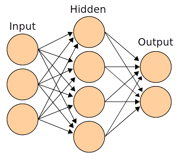
Let’s think that we are trying to build an image classifier that can predict what an image is . We use supervised learning for solving this. Given a color image (RGB image) which consists of D = W X H X 3 (color depth = 3) be stored as an array .We assume that there are “n” categories to be classified into.The task is to come up with a function which classify our image as being one of “n” images.
To build this we start with a set of previously classified labeled “training data”. We can use a simple linear activation function [F(x,W,b) = Wx +b] for score function.W — matrix of size n X D called weights and vector b of size n X 1 called biases. To predict probability for each category , we pass this output through something called a softmax function σ that squashes the scores to a set of numbers between 0 and 1 that add up to 1. Let’s suppose our training data is a set of N pre-classified examples xi∈ℝD, each with correct category yi∈1,…,K. To determine the total loss across all these examples is the cross entropy loss:
L(s)=−∑i log(syi)
For the optimization part ,we use gradient descent. We have to find weights and biases that minimizes this loss.
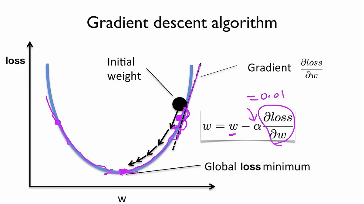
Our aim here is to find the global loss minimum which is at the bottom of the curve. We also use a parameter called the learning rate(α), which is a measure of how fast we modify our weights.
Summing it all up, initially we gave some image as a raw array of numbers, we have a parameterised score function (linear transformation followed by a softmax function) that takes us to category scores. We have a way of evaluating its performance (the cross entropy loss function). Then we improve the classifier’s parameters (optimisation using gradient descent). But here the accuracy is less , therefore we use Convolutional Neural Networks to improve accuracy.
Basics of Convolutional Neural Network(CNN)
Previously we used linear score function ,but here we will use non-linear score function.For this we use neurons which are functions which first multiplies each of its inputs by a weight and sums these weighted inputs to a single number and adds a bias. It then passes this number through a nonlinear function called the activation and produces an output.

Normally to improve the accuracy of our classifier, we’d probably think that it is easy to do so by adding more layers to our score function.But there are some problems to that -
1. Generally, neural networks entirely disregard the 2D structure of the image . For example if we are working with the input image as a 30×30 matrix, they worked with the input as a 900 number array. And you can imagine there is some useful information in pixels sharing proximity that’s being lost.
2. Number of parameters we would need to learn grows really rapidly as we add more layers.
To solve these problems , we use convolutional neural networks.
Difference between normal networks and CNN is that instead of using input data as linear arrays, it uses input data with width, height and depth and outputs a 3D volume of numbers. What one imagines as a 2D input image (W×H) gets transformed into 3D by introducing the colour depth as the third dimension (W×H×d). (it is 1 for greyscale and 3 for RGB.) Similarly what one might imagine as a linear output of length C is actually represented as 1×1×C. There are two layer types which we use -
1. Convolutional layer
The first is the convolutional (Conv) layer. Here we have a set of filters. Let’s assume that we have K such filters. Each filter is small , with an extent denoted by F and has depth value of its input. e.g. A typical filter might be 3×3×3 (3 pixels wide and high, and 3 from the depth of the input 3-channel color image).
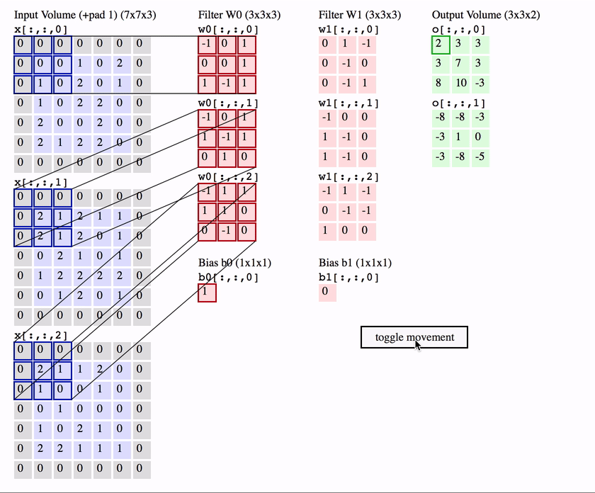
We slide the filter set over the input volume with a stride S that denotes how fast we move. This input can be spatially padded (P) with zeros as needed for controlling output spatial dimensions. As we slide, each filter computes dot product with the input to produce a 2D output, and when we stack these across all the filters we have in our set, we get a 3D output volume.
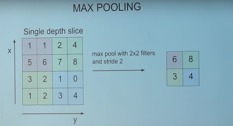
2. Pooling layer
Its function is to progressively reduce the spatial size of the representation to reduce the amount of parameters and computation in the network. It does not have any parameters to learn.
For example, a max pooling layer with a spatial extent F=2 and a stride S=2 halves the input dimensions from 4×4 to 2×2, leaving the depth unchanged. It does this by picking the maximum of each set of 2×2 numbers and passing only those along to the output.
This wraps up fundamentals and I hope you have got the idea about the basic workings.
Let’s begin !
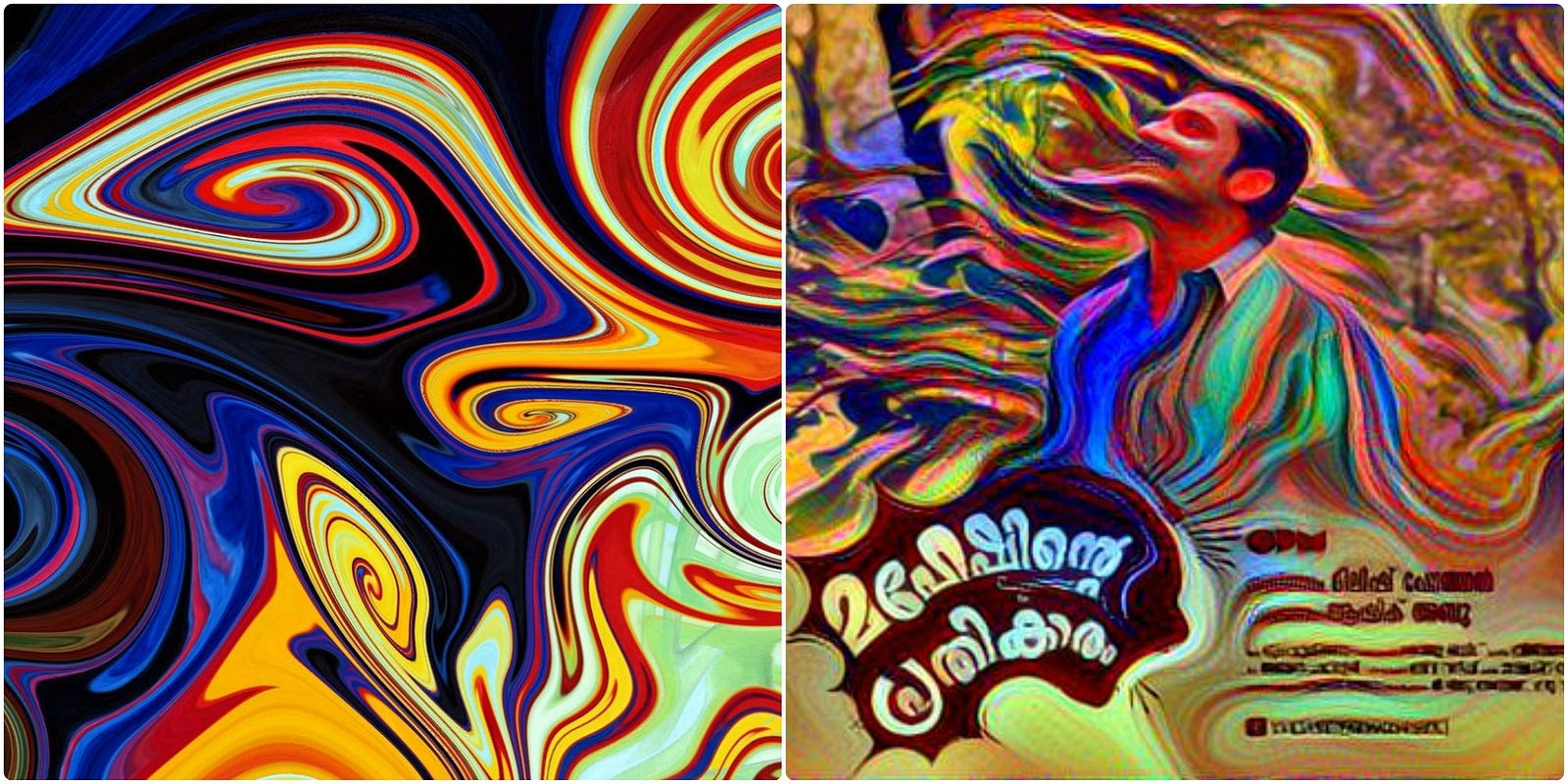
Content image and style image
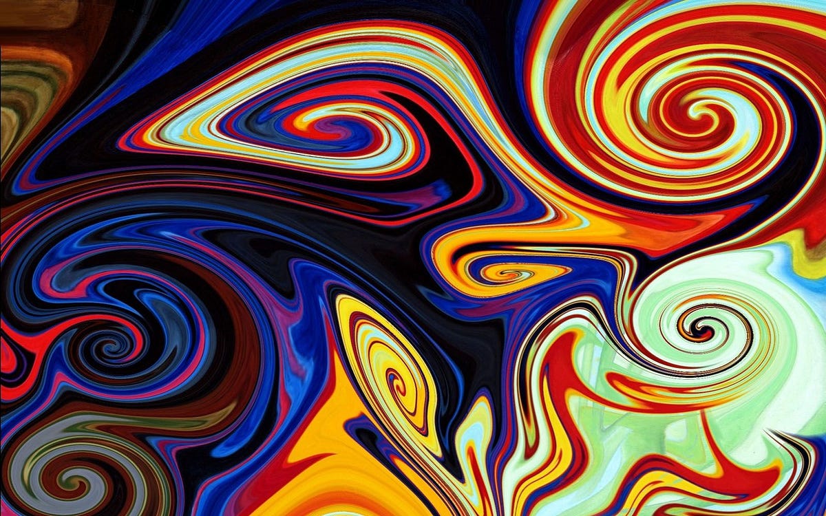
Content image (c) is the image that you would want to be re-create. It provides the main content to the new output image. It could be any image of a dog, a selfie or almost anything that you would want to be painted in a new style. Style image (s) on the other hand provides the artistic features of an image such as pattern, brush strokes, color, curves and shapes. Let’s call the style transferred output image as x.
Loss functions
Lcontent(c,x) : Here our aim is to minimize loss between content image and output image, which means we have a function that tends to 0 when its two input images (c and x) are very close to each other in terms of content, and grows as their content deviates. We call this function the content loss.
Lstyle(s,x): This is the function which shows how close in style two images are to one another. Again, this function grows as its two input images (s and x) tend to deviate in style. We call this function the style loss.
Now we need to find an image x such that it differs little from content image and style image.
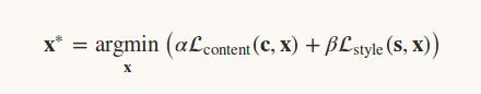
α and β are used to balance the content and style in the resultant image.
Here we will be using VGGNet which is a CNN-based image classifier which has already learnt to encode perceptual(e.g., stroke size,spatial style control, and color control) and semantic information that we need to measure these semantic difference terms.
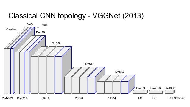
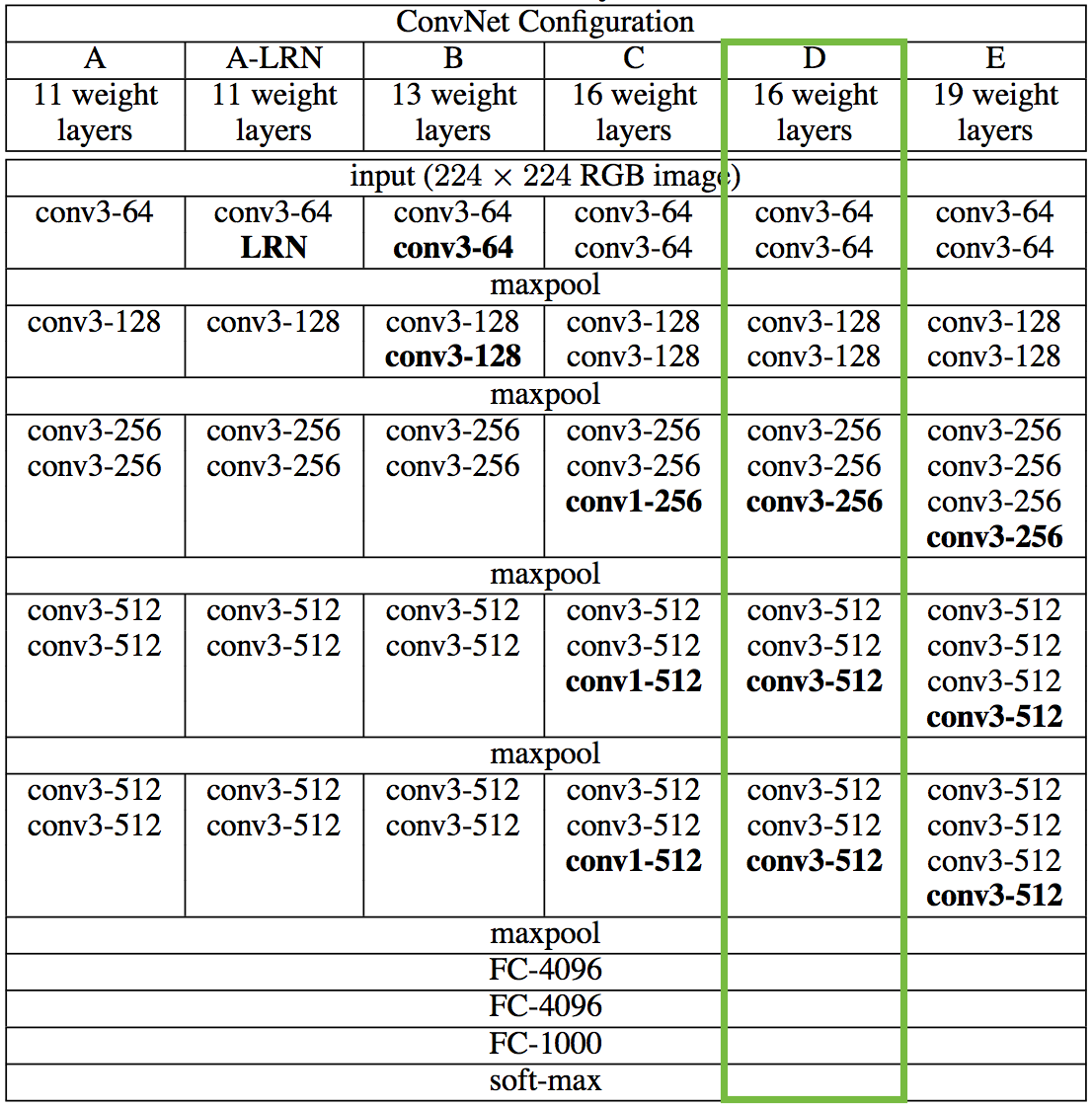
VGGNet considerably simplified the ConvNet design, by repeating the same smaller convolution filter configuration 16 times: All the filters in VGGNet were limited to 3×3 , with stride and padding of 1, along with 2×2 maxpooling filters with stride of 2.
We’re going to first reproduce the 16 layer variant marked in green for classification, and in the next notebook we’ll see how it can be repurposed for the style transfer problem.
Normal VGG takes an image and returns a category score, but here we take the outputs at intermediate layers and build Lcontent and Lstyle. Here we don’t include any of the fully-connected layers.
Let’s get coding ,
Import the necessary packages.
from keras.applications.vgg16 import preprocess_input, decode_predictions
import time
from PIL import Image
import numpy as np
from keras import backend
from keras.models import Model
from keras.applications.vgg16 import VGG16
from scipy.optimize import fmin_l_bfgs_b
from scipy.misc import imsave
Load and preprocess the content and style images
height = 450
width = 450
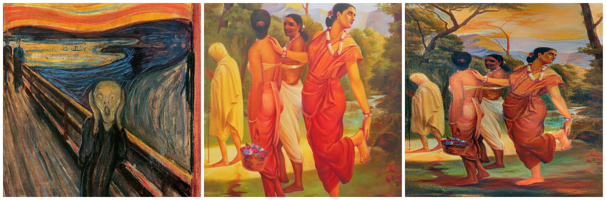
content_image_path = 'images/styles/SSSA.JPG'
content_image = Image.open(content_image_path)
content_image = content_image.resize((width, height))
style_image_path = 'images/styles/The_Scream.jpg'
style_image = Image.open(style_image_path)
style_image = style_image.resize((width, height))
Now we convert these images into a suitable form for numerical processing. In particular, we add another dimension (beyond height x width x 3 dimensions) so that we can later concatenate the representations of these two images into a common data structure.
content_array = np.asarray(content_image, dtype='float32')content_array = np.expand_dims(content_array, axis=0)style_array = np.asarray(style_image, dtype='float32')style_array = np.expand_dims(style_array, axis=0)
Now we need to compress this input data to match what was done in “Very Deep Convolutional Networks for Large-Scale Image Recognition” , the paper that introduces the VGG Network .
For this, we need to perform two transformations:
1. Subtract the mean RGB value (computed previously on the ImageNet training set and can be obtained from Google searches) from each pixel.
2. Change the ordering of array from RGB to BGR .
content_array[:, :, :, 0] -= 103.939content_array[:, :, :, 1] -= 116.779content_array[:, :, :, 2] -= 123.68content_array = content_array[:, :, :, ::-1]style_array[:, :, :, 0] -= 103.939style_array[:, :, :, 1] -= 116.779style_array[:, :, :, 2] -= 123.68style_array = style_array[:, :, :, ::-1]
Now we’re ready to use these arrays to define variables in Keras backend . We also introduce a placeholder variable to store the combination image that retains the content of the content image while incorporating the style of the style image.
content_image = backend.variable(content_array)style_image = backend.variable(style_array)combination_image = backend.placeholder((1, height, width, 3))
Finally, we concatenate all this image data into a single tensor which is suitable for processing by Keras VGG16 model.
input_tensor = backend.concatenate([content_image,style_image,combination_image], axis=0)
The original paper uses the 19 layer VGG network model from Simonyan and Zisserman (2015), but we’re going to instead follow Johnson et al. (2016) and use the 16 layer model (VGG16) . Since we are not interested in image classification , we can set include_top=False so that we don’t include any of the fully-connected layers.
model = VGG16(input_tensor=input_tensor, weights='imagenet',include_top=False)
The loss function we want to minimise can be decomposed into content loss, style loss and the total variation loss.
The relative importance of these terms are determined by a set of scalar weights. The choice of these values are up to you , but the following have worked better for me
content_weight = 0.050style_weight = 4.0total_variation_weight = 1.0
For the content loss, we draw the content feature from block2_conv2.The content loss is the squared Euclidean distance between content and combination images.
def content_loss(content, combination):
    return backend.sum(backend.square(combination - content))
layer_features = layers['block2_conv2']
content_image_features = layer_features[0, :, :, :]
combination_features = layer_features[2, :, :, :]loss += content_weight * content_loss(content_image_features,
combination_features)For the style loss, we first define something called a Gram matrix. Gram matrix of a set of images which represents the similarity or difference between two images. If you have an (m x n) image, reshape it to a (m*n x 1) vector. Similarly convert all images to vector form and form a matrix ,say, A.
then the gram matrix G of these set of images will be
G = A.transpose() * A;
Each element G(i,j) will represent the similarity measure between image i and j.
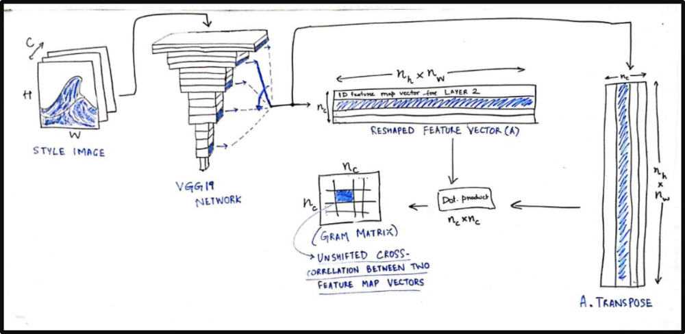
def gram_matrix(x):features = backend.batch_flatten(backend.permute_dimensions(x, (2, 0, 1)))gram = backend.dot(features, backend.transpose(features))return gram
We obtain the style loss by calculating Frobenius norm(It is the matrix norm of a matrix defined as the square root of the sum of the absolute squares of its elements) of the difference between the Gram matrices of the style and combination images.
def style_loss(style, combination):
    S = gram_matrix(style)
    C = gram_matrix(combination)
    channels = 3
    size = height * width
    return backend.sum(backend.square(S - C)) / (4. * (channels ** 2) * (size ** 2))

feature_layers = ['block1_conv2', 'block2_conv2',
                  'block3_conv3', 'block4_conv3',
                  'block5_conv3']
for layer_name in feature_layers:
    layer_features = layers[layer_name]
    style_features = layer_features[1, :, :, :]
    combination_features = layer_features[2, :, :, :]
    sl = style_loss(style_features, combination_features)
    loss += (style_weight / len(feature_layers)) * sl
Now we calculate total variation loss ,
def total_variation_loss(x):a = backend.square(x[:, :height-1, :width-1, :] - x[:, 1:, :width-1, :])b = backend.square(x[:, :height-1, :width-1, :] - x[:, :height-1, 1:, :])return backend.sum(backend.pow(a + b, 1.25))loss += total_variation_weight * total_variation_loss(combination_image)
Now we have our total loss , its time to optimize the resultant image.We start by defining gradients ,
grads = backend.gradients(loss, combination_image)
We then introduce an Evaluator class that computes loss and gradients in one pass while retrieving them using loss and grads functions.
outputs = [loss]outputs += gradsf_outputs = backend.function([combination_image], outputs)def eval_loss_and_grads(x):x = x.reshape((1, height, width, 3))outs = f_outputs([x])loss_value = outs[0]grad_values = outs[1].flatten().astype('float64')return loss_value, grad_valuesclass Evaluator(object):def __init__(self):self.loss_value = Noneself.grads_values = Nonedef loss(self, x):assert self.loss_value is Noneloss_value, grad_values = eval_loss_and_grads(x)self.loss_value = loss_valueself.grad_values = grad_valuesreturn self.loss_valuedef grads(self, x):assert self.loss_value is not Nonegrad_values = np.copy(self.grad_values)self.loss_value = Noneself.grad_values = Nonereturn grad_valuesevaluator = Evaluator()
This resultant image is initially a random collection of pixels, and we use the fmin_l_bfgs_b() function (Limited-memory BFGS (L-BFGS or LM-BFGS) is an optimization algorithm) to iteratively improve upon it.
x = np.random.uniform(0, 255, (1, height, width, 3)) - 128.

iterations = 10

for i in range(iterations):
    print('Start of iteration', i)
    start_time = time.time()
    x, min_val, info = fmin_l_bfgs_b(evaluator.loss, x.flatten(),
                                     fprime=evaluator.grads, maxfun=20)
    print('Current loss value:', min_val)
    end_time = time.time()
    print('Iteration %d completed in %ds' % (i, end_time - start_time))
To get back output image do the following
x = x.reshape((height, width, 3)) x = x[:, :, ::-1] x[:, :, 0] += 103.939 x[:, :, 1] += 116.779 x[:, :, 2] += 123.68 x = np.clip(x, 0, 255).astype('uint8')image_final= Image.fromarray(x)
The resultant image is available in the image_final.
Conclusion
This project will give you a broad idea about the working of CNN and clarify a lot of basic doubts. In this series of articles we will explore the various ways in which deep learning can be used for creative purposes.
Thank you for your time !
Reference:
- http://cs231n.stanford.edu/
- ( Neural Style Transfer: A Review) https://arxiv.org/pdf/1705.04058.pdf
- http://cs231n.github.io/
- (A Neural Algorithm of Artistic Style) https://arxiv.org/pdf/1508.06576.pdf
- http://bangqu.com/0905b5.html
每天推荐一个 GitHub 优质开源项目和一篇精选英文科技或编程文章原文,欢迎关注开源日报。交流QQ群:202790710;微博:https://weibo.com/openingsource;电报群 https://t.me/OpeningSourceOrg